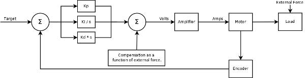
When an external force is applied to a system, standard PID parameters may not be sufficient to compensate for it. To better understand how to address this problem, four applications with external forces will be analyzed and an effective solution will be provided for each application. These applications include servo motors moving a vertical load, a spring load, a lever arm, and a compressible substance.
Vertical Load
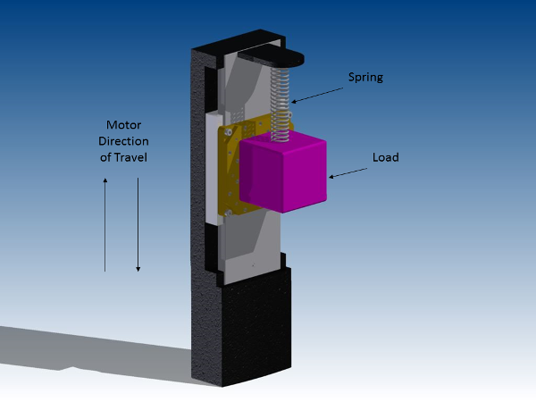
The first application examines a motion controller with an amplifier, and a linear servo motor with a vertical load. The motor and load are mounted vertically. As the motor moves the load, gravity exerts a force pulling the load downward. This gravitational force makes tuning and system stability a challenge.
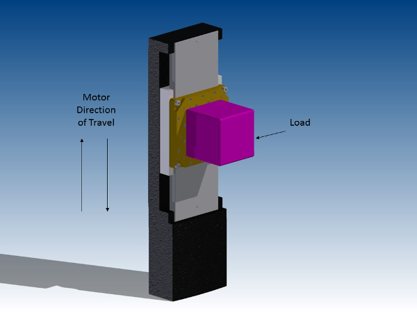 Figure 2. Vertical Load Application
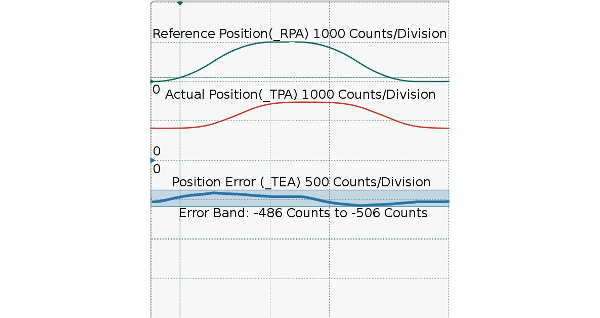
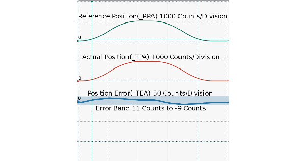
Figure 3 shows the performance of the system with the standard PID tuning parameters. As the load has a fixed mass and gravity is a constant uniform force, a fixed open loop offset can be used to counteract the downward force and improve the performance of the system. The counteracting force can be calculated by using the known mass of the load and the force of gravity. With a 2-kilogram (kg) mass (m) the total amount of force in Newtons (N) to keep the load in place vertically is given by equation (1).
Equation 1
Equation 2
A 19.6 N force is required to counteract the force of gravity. With a gain of 1 Amp/Volt the amplifier will produce 1 Amp of current for every 1 Volt commanded by the controller. The motor has a Force Constant of 11 N/Amp. The current required to produce a 19.6 N force can be calculated as:
Equation 3

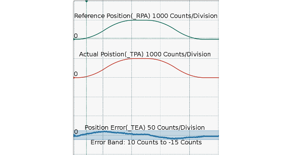
With a gain of 1 Amp/Volt the calculated offset voltage is 1.78 Volts. This value can also be derived from trial and error. Another alternative approach is to command the motor to move back and forth multiple times and take the average torque. Applying the open loop offset will reduce the position error and provide greater stability during moves. By applying the open loop compensation, the position error of the system is greatly reduced, as shown in Figure 4.
Spring Load
In this second application, the setup is the same as previous vertical load, but the motor has a spring connected to the load with a 1 micrometer (μm) resolution encoder. In this situation, the external forces on the load include gravity and the spring. Unlike gravity, the force applied by the spring is not uniform. The force applied by the spring is dynamic, and will vary based on the position of the spring. This means a fixed open loop compensation will not adequately counteract the effect of the spring.
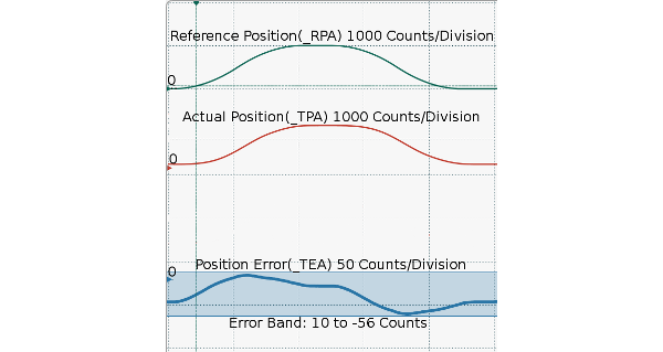
The performance of the system without compensation is shown in Figure 6 below.
To determine the compensation required, the physical behavior of the spring has to be characterized. A spring, having a linear force vs position. The spring’s force in this system can be characterized by the following equation:
Equation 4

In equation (4), F is the force applied by the spring, K is the spring constant, x is the position of the spring, F_P is the spring pre-loading constant to account for compression, and F_G is the force required to counter act gravity. The value for the spring constant K is provided by the spring manufacturer. For the spring used in this application has a spring constant as follows:
Equation 5
When the spring is pre-loaded it will move a distance of 5 mm. By using the spring constant K and the pre-loaded distance traveled for the spring d, the spring preload F_P can be calculated as:
Equation 6
Equation 7
The force to counteract gravity F_G was already calculated with equations (1) and (2) with a result of 19.6 N. With the position of the motor reported in encoder counts (cts) equation (4) now becomes:
Equation 8
Using equation (3), current gain of 1 Amp/Volt, and the motor force constant of 11 N/Amp:
Equation 9

This equation allows the controller to generate a voltage that is directly proportional to the counteracting force F (in N). The commanded voltage changes dynamically as the spring compresses and extends. With the equation providing compensation for the spring, the position error is reduced for the system. This can be seen with the lower position error shown in Figure 7.
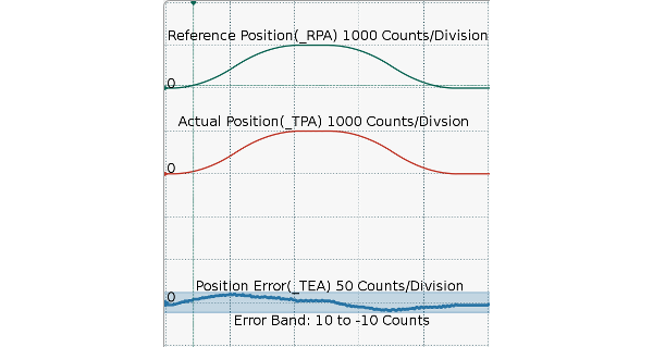 Figure 7. Performance with spring compensation applied
Lever Arm
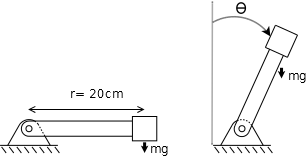
In this example the system has a motor, a motion controller with an amplifier, and a lever arm with a mass at the end. Due to the lever arm’s mechanics, the effective force of gravity will vary as the arm travels from 0 to 90 degrees as shown in Figure 8.
The torque on the motor can be described with equation (2):
Equation 10

Where T is the additional moment applied, r is the lever arm length, θ is the angle (0° being vertical) and m is the mass of the object. Assuming the lever arm itself has negligible mass, the force required to counteract gravity can be calculated dynamically. With a mass of 1 kg and a length of 20 cm, the equation (2) becomes:
Equation 11

The angle Θ is calculated by converting the motor’s position in encoder counts into degrees. This can be done by using the conversion factor. The motor has an encoder that is 4000 cts per revolution and is connected to the lever arm. One full revolution of the motor results in one full revolution of the lever arm.

After conversion equation (11) becomes:
Equation 12

Where Θ is the position in cts.
The motor has a torque constant (K_T) of 5 Nm/A , the torque for a motor can be expressed with equation (13).
Equation 13
Solving equation (13) for A produces equation (14)
Equation 14
Using equation (11) and the motor torque constant (K_T), equation (14) becomes:
Equation 15

With an amplifier gain of 1 A/V, the controller applies a voltage directly proportional to counteracting force of magnitude T in N*m. This improves the system’s overall performance and reduces position error. Figure 9 shows the performance without applying the compensation, and Figure 10 shows the improvements by applying compensation.
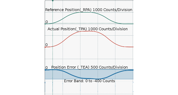 Figure 9 – Lever Arm System performance without compensation
Compressible Substance
In this final application, there is a linear motor connected to a motion controller with an amplifier. The motor is moving an apparatus that is compressing a viscous substance. As the substance is compressed it generates a variable pressure force that pushes back against the motor. As the volume of the substance decreases, the overall pressure against the motor will increase. Unlike the spring, the substance’s response is not linear. In order to oppose this external force the motor must apply a counteracting force that changes dynamically based on the motor position.
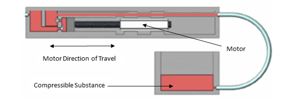 Figure 11. Compressible Substance Application
By assuming a constant operating temperature, the ideal gas law equation (16) can be used to model the pressure applied to the motor.
Equation 16

Where:
P=Pressure (Pa)
V=Volume (L)
n=Amount of substance (mol)
R=Ideal gas constant (kgm2mol-1K-1S-2)
After making multiple measurements on the substance, the data is recorded into Table
1. This data characterizes the pressure force for different positions of the motor.
| Position in Encoder Counts | Force in Newtons |
| 400 | 0.15 |
| 800 | 0.21 |
| 1200 | 0.23 |
| 1600 | 0.29 |
| 2000 | 0.4 |
| 2400 | 0.5 |
| 2800 | 0.6 |
| 3200 | 0.8 |
| 3600 | 1.2 |
| 4000 | 1.8 |
Table 1. Substance Pressure Data
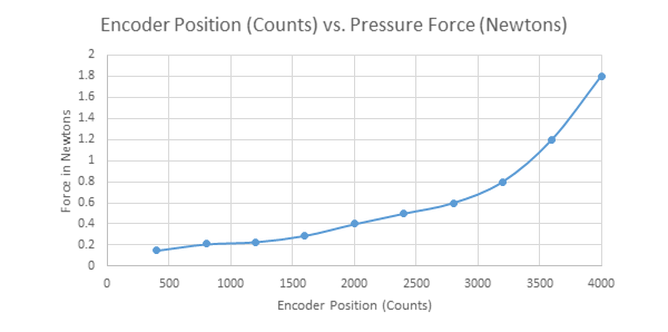
The data from Table 1 is then entered into the controller’s memory as an array. With the array data, the controller can calculate the amount of force required to oppose pressure with the equation (10):
Equation 17
Where:
Equation 15
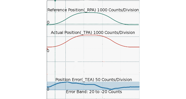
m is the difference between two points in the array data and X is the motor’s current position in Counts. Calculating m and X allows the controller to interpolate between the Table 1 data points to dynamically determine the offset Y. Based on the data available b can also be determined. The controller will apply an offset of magnitude Y to counteract the pressure. The resultant system performance before applying an offset is shown in Figure 14.
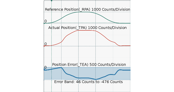 Figure 13 – Compressible Substance system performance without compensation
Effective Solutions
The effects of external forces can be addressed by various methods. In each of the preceding examples the affect an external force was reduced by commanding a corrective force from the motor. This corrective force was calculated using multiple methods including an equation, formula, and data table. Using these methods with the available tuning parameters allows the Galil controller to deliver accurate and stable motion in any application with external forces.