 The Tuning & System Evaluation Tool
Description
The Tuning & System Evaluation tool is used for tuning feedback loops on Galil motion controllers and PLCs and evaluating their performance. It allows easy access to the control filter, includes various auto-tuning algorithms for various situations, and includes evaluation algorithms to evaluate the system performance.
Safety while Tuning and Evaluating
An improperly tuned feedback loop can result in instability and other undesirable motion or plant behavior.
Click the Abort ![]() button on the Tuning & System Evaluation tool to send
AB;MO to
disable
the feedback loop.
button on the Tuning & System Evaluation tool to send
AB;MO to
disable
the feedback loop.
By default, the tuning algorithms provided in the Tuning & System Evaluation tool disable the motors after tuning. This is to prevent the axis from overheating or going unstable if the system is left unattended after the tuning algorithm is complete. This option can be deselected to allow the motor to stay enabled after the tuning algorithm.
Note: The motor is automatically enabled when executing a System Evaluation.
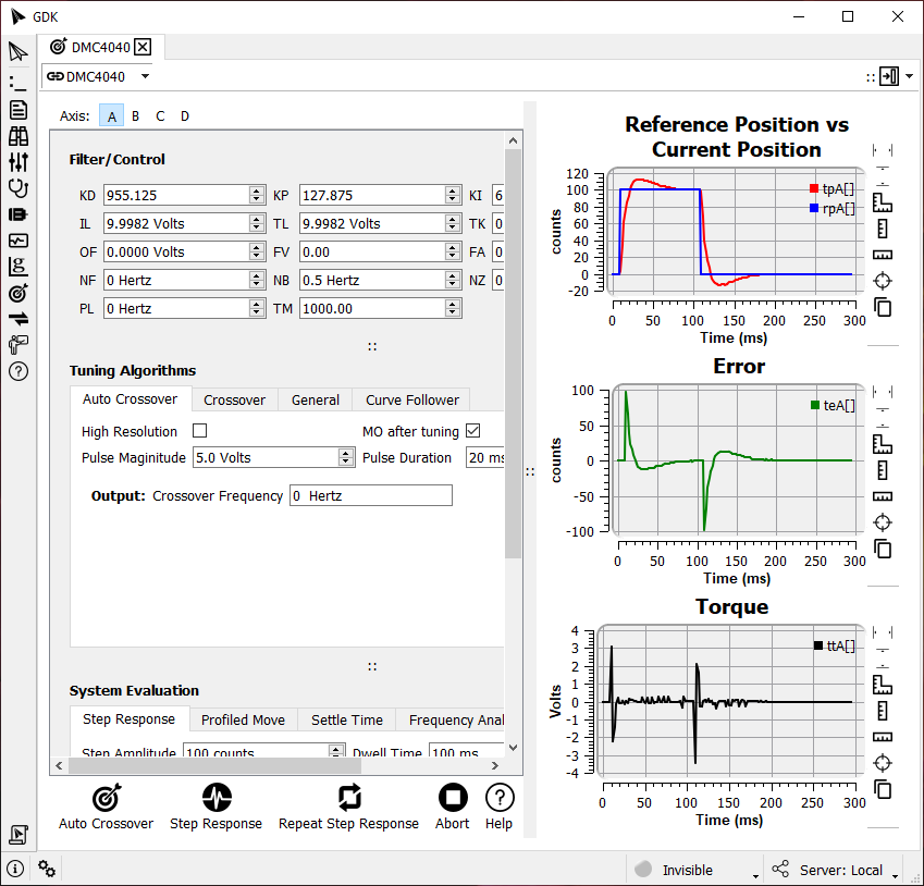
User Interface
The upper left corner of the tool has a row of letters where the user can select which axis to tune or evaluate. The tool is then laid out into two main sections: inputs on the left and plots on the right. The inputs can be collapsed for a larger view of the plots.
The inputs are split into 3 panels: Filter/Control at the top, Tuning Algorithms in the middle, and System Evaluation at the bottom. Each panel can be collapsed individually if desired, and they contain inputs that can be edited.
In the bottom left corner of the window is a panel of buttons. Starting from the left, the first button
![]() Run Tuner executes the displayed tuning algorithm. The second
button
Run Tuner executes the displayed tuning algorithm. The second
button ![]() Run Evaluation runs the
displayed system evaluation. The third button
Run Evaluation runs the
displayed system evaluation. The third button ![]() Repeat Evaluation
runs the displayed system evaluation at
regular intervals. This interval can be adjusted in GDK's settings under the Tuning & System Evaluation tab.
The fourth button
Repeat Evaluation
runs the displayed system evaluation at
regular intervals. This interval can be adjusted in GDK's settings under the Tuning & System Evaluation tab.
The fourth button ![]() Abort will abort the active algorithm or
evaluation and send the AB;MO
command to the controller.
Abort will abort the active algorithm or
evaluation and send the AB;MO
command to the controller.
Note: The Tuning Algorithms sub-section and button are removed for controllers with ceramic firmware.
Filter/Control
The top panel of the inputs contains all of the parameters on the motion controller that can be adjusted for tuning the feedback loop. They are displayed as two-letter DMC commands that apply to the selected axis. Each command can be hovered over to bring up a tooltip with the command's full name, and they are described in the motion controller's command reference.
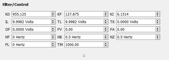
These parameters are updated live. User input is transmitted directly to the controller. If the setting is changed via another source, e.g. an auto-tuner, the panel will update in real time.
Note: TM is a global parameter that affects all axes on the controller. Check your controller's respective documentation on the effects of changing TM.
Tuning Algorithms
Tuning can often be greatly simplified by using one of Galil's Tuning algorithms found in the center input panel.
Open the Tuning Algorithms panel to view the available algorithms for the
current controller. Modify the algorithm properties as needed and click the
![]() Run Tuner button at the bottom left corner of the window to
initiate
the algorithm. All inputs will be grayed out until the algorithm is complete. A
popup will indicate that the algorithm has finished and ask if the displayed
System Evaluation should be executed. Tuning algorithms do not populate
plots on the right-hand window. Only system evaluations populate the plots.
Run Tuner button at the bottom left corner of the window to
initiate
the algorithm. All inputs will be grayed out until the algorithm is complete. A
popup will indicate that the algorithm has finished and ask if the displayed
System Evaluation should be executed. Tuning algorithms do not populate
plots on the right-hand window. Only system evaluations populate the plots.
Each tuning algorithm is described below:
- Auto-Crossover: This algorithm should be used for most axes that use a torque mode amplifier or follow a similar control model. It evaluates an appropriate crossover frequency and applies the corresponding PID filter for the axis. The “Pulse Magnitude” and “Pulse Duration” inputs determine the magnitude and duration of the impulse signal used to measure the axis characteristics. They should be significant enough to engage motion in all of the mechanical components for that axis.
- Crossover: This algorithm is for more advanced users who want to tune their axis to a specific crossover frequency. It is identical to the Auto-Crossover algorithm, except it configures the PID filter based on the user-specified crossover frequency.
- General: This algorithm can be used for axes with a variety of configurations, such as an axis with a
velocity mode amplifier. It determines the stiffest PID filter that can be applied while maintaining axis
stability, and it can take approximately 15 minutes to finish depending on the axis.
- The “Step Size” indicates the move distance in the algorithm. It should be large enough to engage motion in all mechanical components on the axis.
- The “Speed”, “Acceleration”, and “Deceleration” should be configured according to the highest the speed, acceleration, and deceleration that is required in the application.
- For KP, KI, and KD, the “Minimum” and “Maximum” determine the range of acceptable values for the PID filter, and the “Increment” determines how much the PID values increment with each iteration of the algorithm.
- Curve Follower: This algorithm should be used to tune axes that must follow a path as closely as
possible. It determines the PID filter that results in the lowest maximum error during a move, using a
sinusoidal move profile as reference. This algorithm can take 30 minutes or more to finish depending on
the axis.
- The “Distance” specifies the amplitude of the move profile. The amplitude should be large enough to engage all motion in all of the mechanical components of the axis
- The “Frequency” determines the frequency of the move profile, and it should be set to generate a speed and acceleration comparable to the top speed and acceleration required in the application.
- For KP, KI, and KD, the “Minimum” and “Maximum” determine the range of acceptable values for the PID filter, and the “Increment” determines how much the PID values increment with each iteration of the algorithm.
Note: All algorithms have a “high resolution” option. This is intended for systems with low inertia coupled with high resolution position feedback. This option should generally be used when the axis's position feedback is finer than 1 micron. If applicable, a popup will indicate recommend changes to the input parameters, and these can be accepted or rejected as needed.
System Evaluation
The bottom input panel is used for evaluating the performance of the feedback loop for the selected axis.
Open the System Evaluation panel to view the available evaluations for the
current controller. Modify the evaluation properties as needed and click the
![]() Run Evaluation button at the bottom left corner of the window to
initiate
the evaluation. All inputs will be grayed out until the algorithm is complete.
The
Run Evaluation button at the bottom left corner of the window to
initiate
the evaluation. All inputs will be grayed out until the algorithm is complete.
The ![]() Repeat Evaluation button runs the displayed system
evaluation at regular
intervals, in which case the inputs can be modified between evaluations.
Repeat Evaluation button runs the displayed system
evaluation at regular
intervals, in which case the inputs can be modified between evaluations.
When the system evaluation is complete, it provides an output in the System Evaluation panel, and it plots the results on the right-hand plot window,
Each system evaluation is described below:
- Step Response: This evaluation is used to push the feedback loop to saturation and characterize the axis as underdamped, overdamped, or stable. It does this by commanding a sudden jolt to a new position, dwelling there for a short period, then commanding another jolt to the original position. The “Amplitude” should be large enough to engage motion in all of the mechanical components of the axis, and the “Dwell time” should be a reasonable amount of time for the axis to settle at a new position. The “Error Limit” determines the maximum amount of error that the axis can sustain to be considered settled. Three plots are shown after evaluation: one comparing the reference (commanded) position against the actual position, one showing the position error, and one showing the torque.
- Profiled Move: This evaluation is used to drive the axis at certain speeds and accelerations and will characterize the axis as underdamped, overdamped, or stable. It does this by commanding a forward move, dwelling there for a short period, then commanding a reverse move to the original position. The speed, acceleration, deceleration, and distance should be comparable to what is required from the application. The dwell time should be a reasonable amount of time for the axis to settle at a new position. The “Error Limit” determines the maximum amount of error that the axis can sustain to be considered settled. Three plots are shown after evaluation: one comparing the reference (commanded) position against the actual position, one showing the position error, and one showing the torque.
- Settle Time: This evaluation measures the time required for the axis to settle to a specified error window. The axis is considered settled when it maintains a position error less than the specified “Error Limit” for a time period specified by “Window Duration”. The evaluation commands a forward and reverse move, then measures the time from the end of the profile until the axis is settled. Two plots are shown after evaluation: One showing the axis velocity over time, and one showing the position error over time. The position error plot will also include a black box representing the error window for both moves, with height and width corresponding to the specified Error Limit and Window Duration.
- Frequency Response: This evaluation is for more advanced users. It excites the axis at various frequencies and measures the amplitude of the response. The response is used to identify system characteristics, such as resonant frequencies. It has an open-loop mode and closed-loop mode, and the user can specify the excitation signal's amplitude and range of frequencies. This evaluation results in two plots per loop type: the top plot for each shows either the actual position against the reference position or error (depending on the loop type), and the bottom shows the system gain at each frequency.
Plots
Each system evaluation will produce plots that can be inspected and interpreted. Each plot will have a legend in the top-right corner indicating the colors corresponding to each signal.
The user can add cursors to each plot ![]() Data Cursor
and
Data Cursor
and ![]() Time Cursor that allow users to inspect
values at certain locations and measure the differences in the time or data axes. The cursor edges can be
dragged with the mouse to the desired locations. The cursors can also be toggled off.
Time Cursor that allow users to inspect
values at certain locations and measure the differences in the time or data axes. The cursor edges can be
dragged with the mouse to the desired locations. The cursors can also be toggled off.
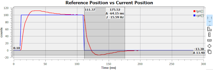
The cursors can also be placed using the “measure” tools ![]() Measure Square Region,
Measure Square Region, ![]() Measure Data Region, and
Measure Data Region, and ![]() Measure Time Region which allow the user to click and
drag the mouse across a region of the plot to have the cursors placed around that region.
Measure Time Region which allow the user to click and
drag the mouse across a region of the plot to have the cursors placed around that region.
There is also the ![]() Track Points tool. When it is toggled
active, the user can click on a
point in the plot to read its position along the time and data axes.
Track Points tool. When it is toggled
active, the user can click on a
point in the plot to read its position along the time and data axes.
The plots also have a ![]() Carbon Copy tool. Toggling this active
saves a copy of the
existing plot that stays visible even if a new system evaluation is performed. The saved copy is overlaid
over any new plots with a lighter color, allowing for easy comparison of performance between runs.
Carbon Copy tool. Toggling this active
saves a copy of the
existing plot that stays visible even if a new system evaluation is performed. The saved copy is overlaid
over any new plots with a lighter color, allowing for easy comparison of performance between runs.
Advanced Data Analysis
The plots in Tuning & System Evaluation Tool have been specially designed to give the best view of the relevant data. However, there may be times when a user need a more in-depth view of a certain plot. In theses cases the scope tool can assist. Since all of the data is recorded in arrays, these can simply be uploaded to the scope where a user can have access to all the scopes features such as zooming, measuring, printing, and more.
![]()